Monte Carlo Simulation for a Skidding Vehicle
The initial speed u of a vehicle sliding to a speed v can be calculated from the equation
Where:
µ = coefficient of friction
u = initial speed
v = final speed
g = acceleration due to gravity ( 9.81ms-2)
s = skidded displacement
If the input data is subject to uncertainty (as is always the case), a Monte Carlo simulation can be used to determine the spread of results. Monte Carlo (MC) simulations randomly sample from the uncertain data to obtain a range of results which can then be analysed to determine the uncertainty in the result. This can be compared with the uncertainty derived from other methods such as the analytical method.
In this particular scenario, uncertainty is assumed in the coefficient of friction, the initial speed and the skidded displacement. Any uncertainty in the acceleration due to gravity is likely to be negligible and is ignored for this scenario.
There are a number of possible distributions of random numbers which will depend on the data involved and the judgement of the investigator as to which distribution is to be preferred. For example it may be that the investigator considers that any value between minimum and maximum extremes is equally likely. In that case a uniform distribution would be preferred. Alternatively a most likely value may be considered with the likelihood of any likely value falling away further from the most likely value. In this case a triangular or PERT distribution could be considered. In this scenario it is assumed that the values are known to be distributed with a 95% certainty around a mean. A suitable distribution in this case will be the normal distribution.
To generate a normal distribution of random numbers, a mean value is required along with the standard deviation describing the uncertainty. If the uncertainty is known to a 95% probability, in order to derive the standard deviation, the uncertainty must be divided by the appropriate Student T table value, which for 95% probabilities is 1.96. In a real-world situation, the value and any uncertainty may be derived directly from multiple measurements, so the standard deviation may be known already.
Final speed:
The final speed is assumed accurate to a 95% probability of ± 0.5 ms-1.
v = 10 ms-1 σv = 0.5 / 1.96 = 0.2551
Displacement:
The displacement is assumed accurate to a 95% probability of ± 0.5 m.
s = 25 m σs = 0.2551
Coefficient of friction:
The coefficient of friction is assumed accurate to a 95% probability of ± 0.25
μ = 0.73 σμ = 0.12755
From the mean values the nominal value can be calculated, i.e.
uNominal = 21.4 ms-1
Monte Carlo method
A suitable number of iterations must be chosen. In this scenario 50 000 iterations generates more than enough data for analysis.
Number of iterations:
n = 50000
To use the Monte Carlo method, it is necessary to create suitable vectors of variables randomly distributed about the mean of each variable. Note that each time a calculation on the document is performed, the vectors are regenerated so that the actual mean of the vector will vary slightly with each calculation.
v1 = {50000} mean(v1) = 10
s1 = {50000} mean(s1) = 24.999
μ1 = {50000} mean(μ1) = 0.73026
Monte Carlo simulation results, together with the mean, standard deviation and 95% probability:
uVec = {50000}
meanU = 21.353
devU = 1.4759
Prob95u = 2.8928
Thus from the MC simulation the result to a 95% level of confidence is
21.35 ± 2.893 ms-1
Analytic method
An alternative method to determine the uncertainty in the result is to use an analytic method. This uses the partial derivative of each variable multiplied by the uncertainty associated with that variable and combines the results to determine the spread of results. In more technical terms, if x is a function, f of at least two other variables, i.e.
then the variance of x, can be approximated using partial derivatives as
There are a few caveats to using this analytical method. These are that is no correlation (or at least negligible) correlation between the uncertainty in the variables and that the uncertainty for each variable can be assumed to follow a normal distribution.
Using this method, the analytical data for scenario are:
dv = 0.4673 dMu = 11.456 dS = 0.33453 dU = 1.468621 Prob95 = 2.8785
So, from the analytical method the overall result is found to be
21.399 ± 2.8785 ms-1
Comparison of results
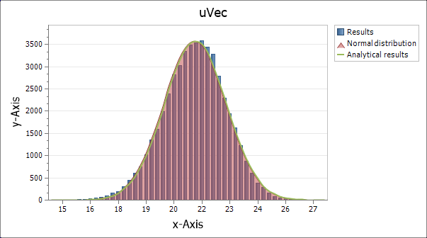
It is impractical to try and display all 50 000 results from this MC simulation on a single graph. To make that data more amenable, the results are collected together into a smaller number of ranges of values found by dividing the total range equally into the required number of ranges. These ranges are known as ‘bins’ or ‘buckets’. This process generates a histogram summarising the results. In SolvePro the function histogram can be used.
The graph below shows a comparison between the results from the MC simulation and the analytical results. A normal distribution curve derived directly from the mean and standard deviation of the MC results is also shown. In SolvePro the function dNorm generates the normal distribution curve.
As can be seen, in this scenario there is a close correlation between all three curves. Depending on the calculation employed, and the assumed distribution of data, the normal distribution of MC results as seen here may not be present and different techniques are required to determine the spread of results.
hist = {2, 50}
normDist = {1, 50}
normDist2 = {1, 50}
histApp = {4, 50}