The Normal Distribution
Generates a vector (series or array) of random numbers distributed according to the normal distribution.
Function definition:
Rnorm(number, mean, sd)
or using symbols,
Rnorm(n, μ, σ)
where
number (n) is the number of values to be generated
mean (μ) is the centre of the distribution
sd (σ) is the standard deviation
Example:
n = 1e+05, μ = 50, σ = 4
vectorNormal = Rnorm(n, μ, σ) = {100000}
The vector can be visualised by first using the Histogram(vector, m) function to sort the vector into a series of ranges of values (bins or buckets)
histNormal = {2, 50}
The histogram can be viewed using the ActiveGraph feature,
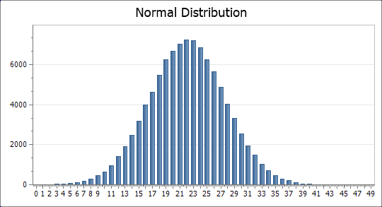
To determine whether the resultant vector has the same mean and standard deviation as defined in the generating function, the Mean(vector) and Stdev(vector) functions can be used.
mean = 50.02 sd = 3.995
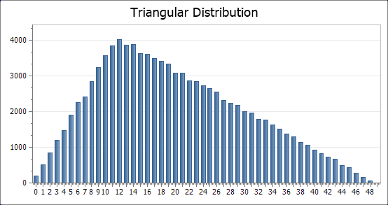
The Triangular Distribution
Generates a vector (series) of random numbers distributed according to the triangular distribution.
Function definition:
Rtri(number, min, max, mode)
where
number is the number of values to be generated
min is the minimum value required
max is the maximum number required
mode is the most likely or ‘best-guess’ value
Example:
n = 1e+05, min = 0, max = 100, mode = 25
vectorTri = Rtri(n, min, max, mode) = {100000}
histTri = {2, 50}
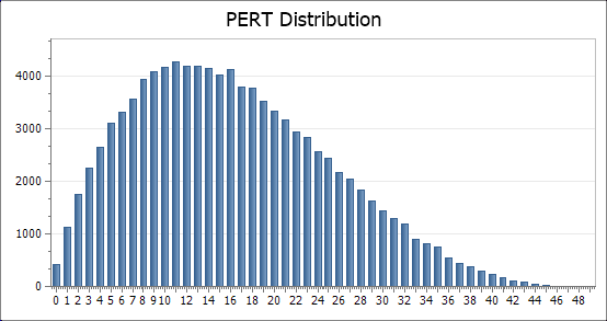
The PERT Distribution
Generates a vector (series) of random numbers distributed according to the PERT distribution. The name is derived from ‘program evaluation and review technique’ for which it was originally developed. PERT distributions are used as an alternative to the triangular distribution as they produce smoother distributions and are likely to better represent subjective knowledge of the data.
Function definition:
Rpert(number, min, max, mode)
where
number is the number of values to be generated
min is the minimum value required
max is the maximum number required
mode is the most likely or ‘best-guess’ value
Example:
n = 1e+05, min = 0, max = 100, mode = 25
vectorPert = Rpert(n, min, max, mode) = {100000}
The vector can be visualised by first using the Histogram(vector, m) function to sort the vector into a series of ranges of values (bins or buckets)
histPert = {2, 50}
The histogram can be viewed using the ActiveGraph feature,
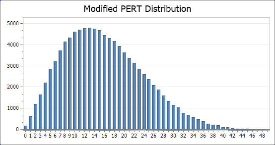
The Modified PERT Distribution
Generates a vector (series) of random numbers distributed according to the modified PERT distribution. The modified PERT distribution introduces a weight parameter which allows control over how much emphasis to place on the mode. The standard PERT distribution uses a fixed value for weight of 4. Lower values place less emphasis on the mode and have the effect of flattening the curve.
Function definition:
Rmpert(number, min, max, mode, weight)
where
number is the number of values to be generated
min is the minimum value required
max is the maximum number required
mode is the most likely or ‘best-guess’ value
weight is the weighting applied to the mode
Example:
n = 1e+05, min = 0, max = 100, mode = 25, weight = 6.5
vectorMPert = Rmpert(n, min, max, mode, weight) = {100000}
The vector can be visualised by first using the Histogram(vector, m) function to sort the vector into a series of ranges of values (bins or buckets)
histMPert = {2, 50}
The histogram can be viewed using the ActiveGraph feature,