
Version 8 of SolvePro introduces a host of new features such as vector processing, charts and graphs as well as enhanced editing tools to make creating a document easier. The enhanced editing tools include a new Styles option to make the creation of headings and text consistent. A variety of built-in and custom tables are also now supported. Both these features follow closely the look of Microsoft Office programs however they do not work in exactly the same way.
Internally, SolvePro now uses numbers containing up to 50 digits. Older versions used the maximum precision available natively in Windows of 16 digits. This means irrational numbers such as √(2) and π can be displayed with more precision if required, e.g.
√(2) = 1.4142135623730950488016887242096980785696718753769
π = 3.1415926535897932384626433832795028841971693993751
More importantly, expressions such (0.1 + 0.2) * 100 are now calculated exactly and generate the result 30. Older versions (and most other programs using standard double floating-point numbers) can in some circumstances display the result as 30.000000000000004 This is due to the way in which decimal numbers are stored and used internally as binary numbers. Decimals such as 0.1 are not represented exactly in binary. Note too that the square root symbol can now be used directly within ActiveEquations.
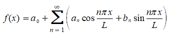
The new EditEquation program is designed for use in SolvePro and can be installed as a separate package. This allows user defined equations to be inserted into your document and edited simply by double clicking on them. An example equation is shown below
Probably the most important and certainly the most powerful feature in version 8 is the ability to process vectors or series of numbers. Using this feature, it is possible to perform the same calculation on a variety of variables each of which can be different for each iteration. This allows for easy processing of ranges of data or more importantly for a series of numbers drawn randomly according to a defined distribution. This allows for simulations to be performed to which can be used to analyse the propagation of uncertainty through the equations. See elsewhere for an in-depth tutorial on creating a Monte Carlo simulation using SolvePro.
Using the new ActiveGraph tool, the results can be displayed graphically and compared with the results from other calculations. For example, the chart below was generated to compare a Monte Carlo simulation of a simple slide to stop calculation, with a propagation of error analysis using partial derivatives.
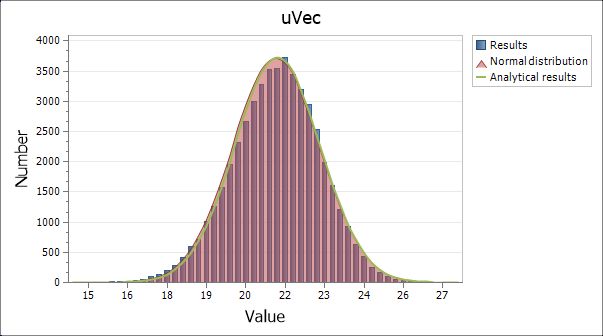
In a SolvePro document, ActiveGraphs really are ‘active’ and respond dynamically to changes in source data. A variety of chart styles are provided, including in 2D points, straight and curved lines as well as areas. Pie and doughnut charts are also available in 2D and in 3D, pie and torus charts. Double clicking on the chart in a document allows the details of the graph to be edited.
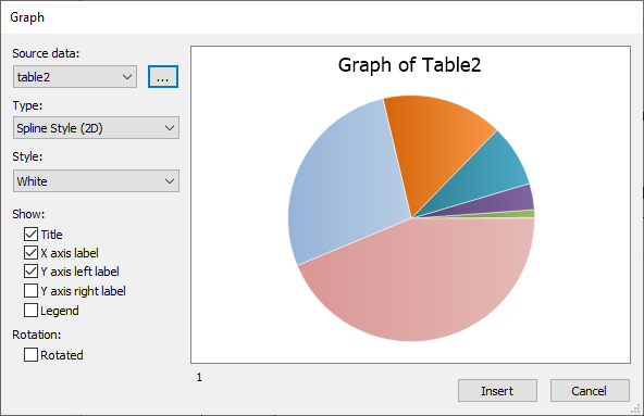
More detailed control of the display and source data can be achieved by clicking on the ellipsis button. See elsewhere for a detailed discussion explaining how to use and control charts and graphs.
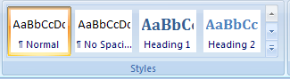
To promote consistency within a SolvePro document, version 8 introduces a series of styles. These are similar to those available in Microsoft Office and allow you to change the style of a paragraph or line of text. The styles are fully customisable and allow the creation of styles such as Title, Heading1, Heading2, Normal, Emphasis etc.
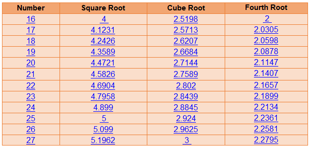
In addition, there is now a fully featured tool to create and maintain tables. Use the Tables command to create a table or the required size and then populate it with whatever data you need to display.
The style and layout of a table can be edited using the controls provided. Rows and columns can be inserted or deleted, individual cells can be merged and then split and, once complete, the overall style can be easily changed. For example, the table below shows a variety of roots to various integers.
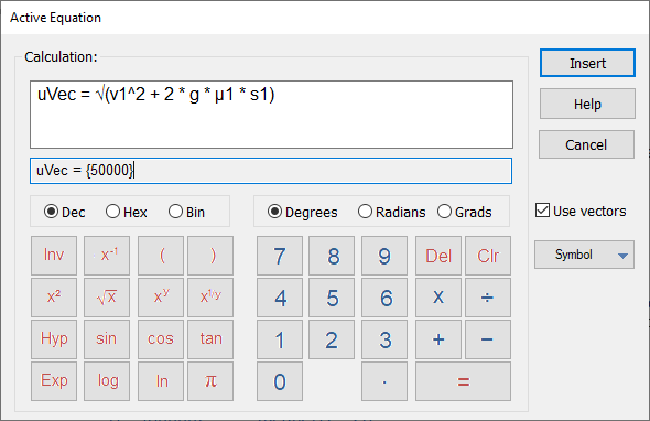
Finally, it is now possible to use Greek symbols as variables and in ActiveEquation objects, so expressions such as v = √(r * μ * g) or c = 2·π·r can be created and used in ActiveEquation objects. To insert Greek and other characters directly into text, the Insert – Symbols command on the View tab can be used.
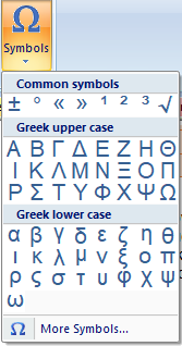
In the ActiveEquation editor, Greek symbols can be inserted using the Symbol drop down box.
We are preparing a series of articles to demonstrate some of the new features and show how to use them and these will be published shortly.